Assignment Details

1. Answer yes or no to each of the items a-c. If yes, briefly justify the statement, if no, provide a counter-example or disprove the statement.

(a) In univariate OLS, depending on whether we use homoskedastic or heteroskedastic standard error, our OLS estimator βˆ1 will be numerically different.

(b) Say Y = β0 + β1X + U but X is endogenous, i.e., cov(X, U) 6= 0. Let Uˆi = Yi − βˆ0 − βˆ1Xi, where (βˆ0, βˆ1) are the usual OLS estimates. Then SU, Xˆ 6= 0.

(c) The problem of perfect multicollinearity can be alleviated by adding more observations to the regression.

2. You are interested in understanding whether student-athletes’ grade point averages (GPAs) suffer during the semester their sport is in season. As such, you have collected data on 366 student-athletes from a large midwestern research university that supports a Division 1 athletics program. Your dataset
includes the following variables:

• termgpa – the student’s GPA for that term, measured on a four-point scale (mean: 2.33)
• sat – the student’s combined SAT score in 100 points
• hsperc – the student’s academic percentile in their high school graduating class
• female – a dummy variable equal to one if the student is female
• season – a dummy variable equal to one if the student’s sport is in season

We will maintain the OLS assumptions throughout this problem. You estimate the following regression using OLS:

termgpa = β0 + β1 log(sat) + β2hsperc + β3hsperc2 + β4female + β5season + β6female ∗ season + U.

You obtain the following estimation results:
termgpa \ = −2.15(.311) + 1.5(.3)log(sat) + .10(.05)hsperc + .20(.04)hsperc2 − .366(.061)female − .035(.07)season +  .05(.005)female ∗ season

(a) What is the interpretation of β1 in this multivariate regression?

(b) You want to test that there is no effect of sport season on student-athletes’ GPAs. Write down your H0 and H1 in terms of (β0, · · ·, β6).

(c) You choose to use F-test to conduct the above test and obtain an F-stat of 5. Use the Chisquare table, is the P-value of your F-test less than 1%, between 1% and 5%, or greater than 5%, and why?

(d) A female student-athlete is median in terms of academic performance in high school (i.e., hsperc = 50% = 0.5). What is the expected increase (in terms of β1, · · ·, β6) of her termgpa if her hsperc increases from 0.5 to 0.7 and the sport changes from offseason (season = 0) to in season (season = 1), given other variables unchanged?

(e) Based on the regression results, what is a valid estimate (number) of the above-expected increase?

(f) In order to construct the confidence interval for the expected increase, you will run an F-test to recover the standard error of the estimator of the expected increase you proposed above. What is the null hypothesis of the F-test you are going to run?

(g) The F-stat you get from the above test is 4. Construct your 95% confidence interval using critical value 1.96.

3. You are interested in the impact of years of education on a woman’s wage. You have collected data from the 1980 U.S. Census on 250,000 married women aged 21-35 with two or more children. Your dataset contains the following variables:

• wage – hourly earning of the woman worked in 1979
• educ – years of education
• proximity – the distance between the individual’s home and the nearest college
• morekids – dummy equal to 1 if the woman has three or more kids
• samesex – dummy equal to 1 if the two oldest children are of the same sex (i.e. boy-boy or girl-girl)

A simple OLS regression of wage on educ yields the following output wage = 21.07(.056) + 5.00(1.00)educ.

(a) Someone told you that your regression suffers from the omitted variable bias. The variable ability is omitted. If that is the case, your current OLS estimate over- or under-estimate the causal effect of education?

(b) You decide to examine whether the level of education is influenced by the distance between the individual’s home and the nearest college. To examine this issue, you regress the variable educ on proximity, yielding the following results educ = .346(.001) + .10(.02)proximity (1)

Do you think proximity is a valid instrument for an IV regression of wage on educ? Why or why not?

(c) What is the (default) F-statistic for regression (1)? Is proximity a weak instrument?

(d) You now estimate the 2SLS regression of wage on educ using proimity as the instrument.

Here are the results: wage = 21.42(.487) + 3.00(1.5) educ

Is the effect of education on wage significant at 5% level (or equivalently, 95 % confidence level)?

(e) You also want to add morekids to the regression and estimate the effect of fertility on women’s wages at the same time. Someone told you that you can use samesex as a valid instrument for more kids. Why it is valid?

(f) So now, you want to regress wage on both educ and morekids, using both proximity and same-sex as IVs. Explicitly describe the two steps when implementing the 2SLS estimation. In particular, describe the regressions you will run in the first and second stages. (Note that in this question, you have two endogenous variables, two IVs, and no controls.)

4. You have a dataset of i.i.d. observations (Yi, Xi), where Yi = β0 + β1Xi + Ui. Suppose the usual OLS assumptions hold. In particular, E(Ui|Xi) = 0.

(a) Prove that EUi = 0 and E(XiUi) = 0.

(b) Note Ui = Yi − β0 − β1Xi. The above two equations imply that E(Yi − β0 − β1Xi) =0

E(Xi(Yi − β0 − β1Xi)) =0.

Then, you propose to estimate β0 and β1 by β˜0 and β˜1 such that they solve the sample version of (2). In particular, β˜0 and β˜1 satisfy

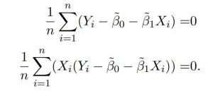
Show β˜0 and β˜1 are consistent estimators of β0 and β1, respectively.

(c) Prove that, for any function of Xi, say f(Xi), Ef(Xi)Ui = 0.

(d) Similar to (2), you have E(Yi − β0 − β1Xi) =0

E(f(Xi)(Yi − β0 − β1Xi)) =0. Following the same idea, you propose the estimators β˘0 and β˘1 such that they solve the sample version of (3):

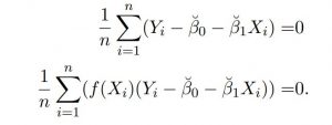
Show that β˘0 and β˘1 are consistent estimators of β0 and β1, respectively.